Mixing up Math: Item Response Theory (part 3)

Last updated on Apr 23, 2021 13 min read

In the previous post, we investigated the claim by Doug Rohrer and colleagues that mixing up math questions has an effect size of about 0.8 on a math test. In the analysis, we assumed that the points scored on the test could simply be added up. We already questioned this assumption when we explored the data visually and found that for one topic, there seemed to be a jump in understanding - students either answered all four item correct or none correct.

Now we no longer assume that student’s understanding of the math can be mapped directly onto the number of points scored. Instead, we model this understanding, or latent ability, with Item Response Theory (IRT). We first explain the basics of this theory and then use it to evaluate the test that was used in the Rohrer study. How to actually use the latent scores is a topic for a later post.

Item Response Theory

The assumption of IRT is that when we for example administer a test, we are not just measuring the points scored, but really care about an underlying latent variable that causes points to be scored. This variable is the true ability $θ$ of the students for the subject at hand. Instead of summing up the points on a test, the number of points gives information about the location $θ$ of a student on the interval where the latent variable lives. The idea of the theory is that questions differ in their capacity to measure this latent ability. In order to make this idea precise we have to look at the model.

Before we do so, we have to discuss two assumptions. First, we assume that a student’s performance on test items are independent of each other. Second, we assume (for now) that the test measures understanding on one dimension. In the case of the Rohrer math test, it was made up of four different topics, so in that sense it is certainly wrong to make this assumption. But then, we are already talking about only math questions. Also, even within a domain of math such as geometry we can always find subtopics. So by this logic we could never really make this assumption. Let’s go with the assumption of unidimensionality for now then and scrutinize it later.

With respect to the data, we have {0,1} observations (a question is answered correctly or not) and so we want to model the probability that a students answers a questions correctly (i.e. scores a 1) based on their latent ability $θ$ . At first glance, this set up sounds like any old logistic regression model (or probit or whatever you like). But the problem is actually quite different from estimating $β$ in ordinary maximum likelihood estimation for logistic models. The reason is that we do not have values of an explanatory variable X, like age or income. So we cannot simply calculate for every X which value of p best explains the {0,1} outcome on the test. This poses hard problems for estimation. We deal with them in a technical note.

Let’s ignore estimation problems for now and assume that we have somehow conjured up some $θ^{'} s$ . This means we are dealing with a standard logistic regression problem. We immediately complicate things again however, by performing a number of transformations that may be familiar from high school algebra. The operations are not as straightforward though, because the logit is not a standard function. The results of the transformations that we discuss below is the addition of the parameters $α_{i}$ and $δ_{i}$ for every test item i. $P (X_{i} = 1 | θ) = \frac{\exp [α_{i} (θ - δ_{i})]}{1 + \exp [α_{i} (θ - δ_{i})]}$ First, the parameter $δ$ simple shifts the curve to the left when an item is easy and to the right if it is hard. This is a simple translation ( $δ$ ,0). More interestingly, we multiply with respect to the y-axis by $a l p h a$ . Below we display results for $α = 1$ (black), $α = 0.5$ (blue) and $α = 3$ (red), to get a feel for this effect, because it is not immediately obvious from the formula.

library(tidyverse)
## create a domain
x<- c(-4:4)
df<-data.frame(x)

# write a function that gives a logistic function with parameter a
map_logit <- function(a,color,s){
  stat_function(fun=function(x) (exp(a*x)/(1 + exp(a*x) )),
                color=color,
                size=1.05)
}
# plot the curves
ggplot(df,aes(x))+
  map_logit(1,"black") +
  map_logit(0.5,"blue") +
  map_logit(3,"red") +
  labs(
    x = quote(theta),
    y = "P(X=1)"
  )

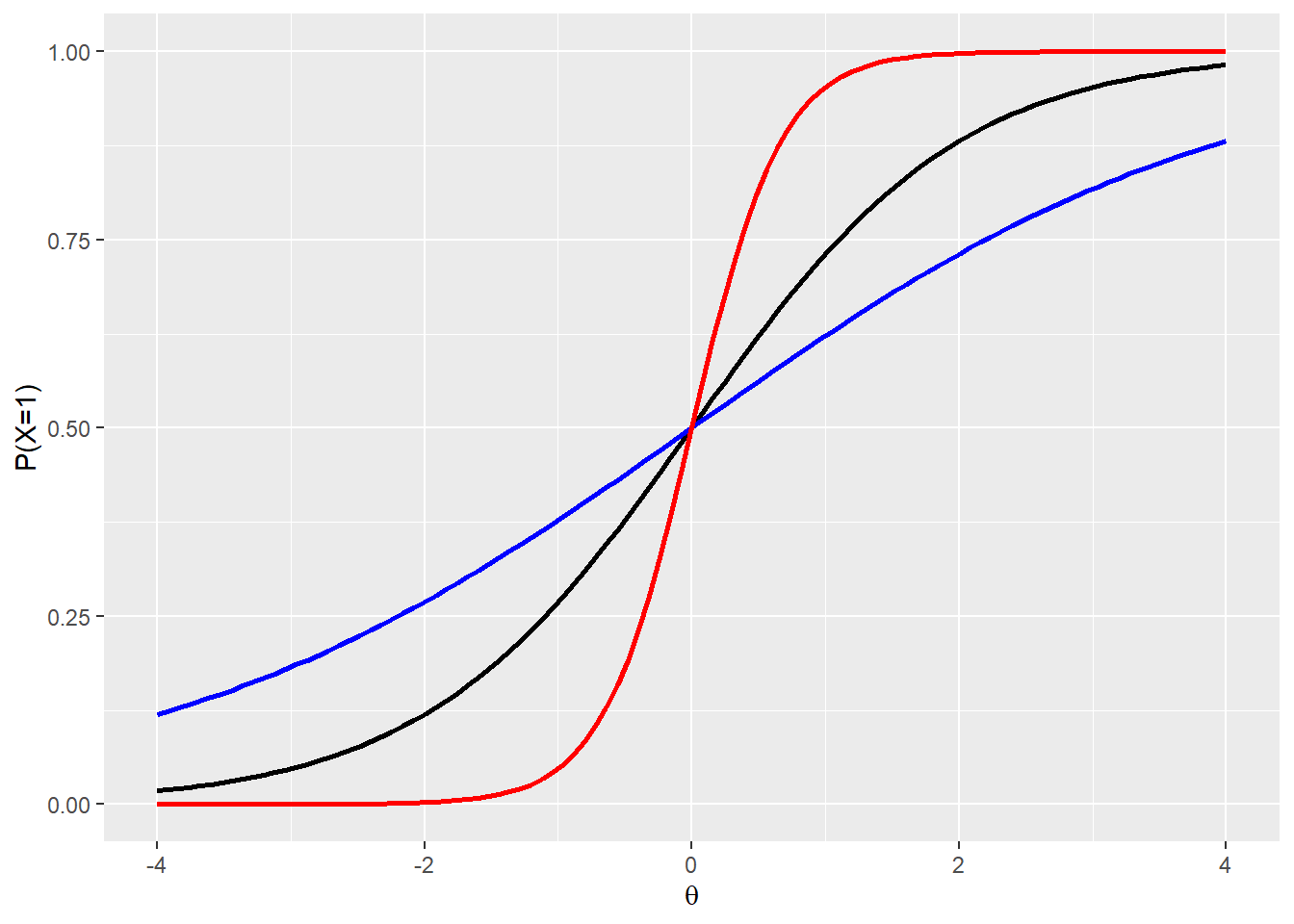
The practical interpretation that we can give is that a bigger $α$ means a test item is more sensitive to difference in ability level $θ$ where it is steep. After all, for the red curve a tiny increase in $θ$ around the average values gives a significant boost to the probability of a correct answer on the item. However, as we move two standard deviations away from the average of $θ$ , the red curve doesn’t do much discrimination any more.

We could also add a parameter $γ$ as a translation (0, $γ$ ) in order to account for guessing, but as we aren’t dealing with multiple choice in the Rohrer test, we won’t consider it here. Because we have two parameters in our model - $α_{i}$ and $δ_{i}$ - we refer to it as a 2PL model.

Technical note

Estimating latent ability scores is a challenge. Let’s have a look at the 2PL model - a logistic model, where we want to estimate the probability of a correct answer given the latent ability and two parameters.

$P (X_{i} = 1 | θ, α, δ) = \frac{\exp [α_{i} (θ - δ_{i})]}{1 + \exp [α_{i} (θ - δ_{i})]}$ The maximum likelihood of $θ$ given the item responses X per person v and item i (where we have J items), is estimated with the following formula. Here $ϕ$ contains both $δ$ and $α$ .

$L_{i} (θ | x_{v}, ϕ) = \prod_{i = 1}^{J} P (X_{v i} = x_{v i} | θ_{v i}, ϕ_{i})$

There surely are a lot of parameters to estimate! So how to go about this? There are several methods.

One is so called joint maximum likelihood estimation. In that case we search for combinations of $θ$ , $δ$ and $α$ that produce a surface ‘above’ them, which gives values of p that maximize the likelihood of all of the {0,1} responses on the test. There is no unique solution to this maximization problem. The technical term is to say that the model is not identified. In order to remedy this shortcoming, the location of a parameter must be fixed and the scale must be fixed. Unfortunately, the resulting estimate is not consistent. This is a technical term that says that no matter how many observations you collect, your estimate is not guaranteed to approach the actual value you are after.

Another solution to estimating parameters on a multivariate distribution is marginal maximum likelihood estimation. Taking the marginal of a multivariate distribution means that you collapse one axis onto the others, so that the probability mass is spread out over this lower dimensional shape. So if we have a two dimensional support below a surface for example, then taking the marginal means that the 3d-object with volume 1 (because of the total probability) is turned into a surface with area 1.

This is what we do here with respect to $θ$ , the latent abilities of the students. The problem is that we cannot integrate out an unknown function. So we have a choice. We either set up some nonparametric distribution for $θ$ that we like, or we come up with some parametric distribution for $θ$ that we like. The standard choice is to choose the normal distribution, with mean 0 and standard deviation 1. Now that $θ$ is gone (for now), we can estimate the maximum likelihood of $p h i$ per test item, based on the data of the students v.

$L (ϕ | X) = \prod_{v} P (x_{v} | ϕ)$ This method requires numerical methods to both integrate and maximize the likelihood. See here for more details on the algorithm used in the mirt package that is dedicated to IRT analyses and is used below.

At this point we will not discuss another alternative, which are Bayesian estimation techniques. See here for a guide.

Once we have estimated the parameters, we find for each person the $θ$ that maximizes the likelihood of their response pattern on the test (i.e. the 0’s and 1’s). The parameters $p h i$ are already estimated and can now weight the contribution of each item to the estimate of the total latent ability level. In the formula below, P stands for the probability that person v gives a correct answer u on item i.

$L (θ_{s} | X_{v}) = \prod_{i = 1}^{J} P_{v i}^{u_{v i}} (1 - P_{v i})^{1 - u_{v i}}$ Note that a high discrimination $a l p h a$ will punish a strongly deviating overall $θ$ estimate more harshly, because the probability on the y-axis reacts stronger. So a high $a l p h a$ will give more weight to an item.

We can also estimate the standard error for an estimate with the so called information function. This is the familiar Fisher information matrix adapted to account for $a l p h a$ and $γ$ , which both influence the sensitivity of the test. For our purposes we fill in $γ$ =0, because we use the 2PL model.

$I n f_{i} (θ) = [α_{i}^{2} \frac{1 - P_{i} (θ)}{P_{i} (θ)}] {[\frac{P_{i} (θ) - γ_{i}}{1 - γ_{i}}]}^{2}$ We can simply add up the information per item to get the test information function - variances can be added after all. $T I n f (θ) = \sum_{i = 1}^{I} I n f_{i} (θ)$ Finally, the standard error is calculated by inverting the square root of the test information function. This should be familiar stuff. $S E (θ) = \frac{1}{\sqrt{T I n f (θ)}}$

Analysis of the Test

Let us now apply the IRT model to the responses on the 16 test items in the Rohrer study. After loading the package mirt and the data, we fit a 2PL model to the data. We plot the graphs for each of the 16 items to check whether our parameters lead to models that fit the data. The data are {0,1} so the dots are binned data, with 95% confidence intervals around them.

# Fit a 1-dim model 
fit1 <- mirt(quest,
             1,                 
             itemtype = '2PL')

# Plot the fit of the models
for (i in 1:length(quest)){
  ItemPlot <- itemfit(fit1,
                      group.bins = 15,
                      empirical.plot = i,
                      empirical.CI = .95,
                      method = 'ML')
  print(ItemPlot)
}

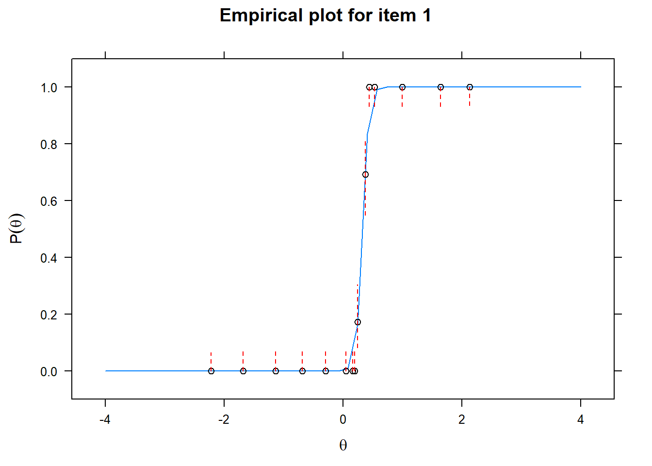
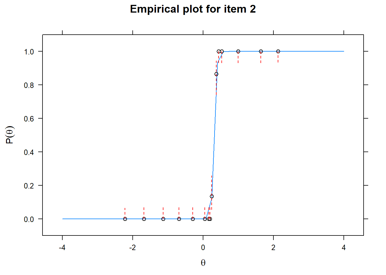
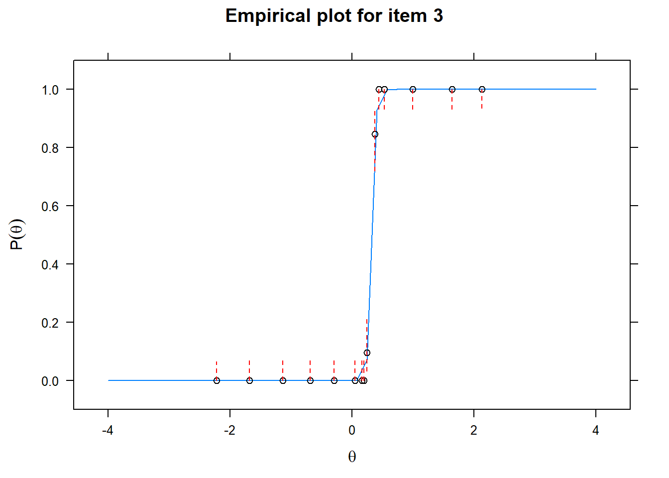
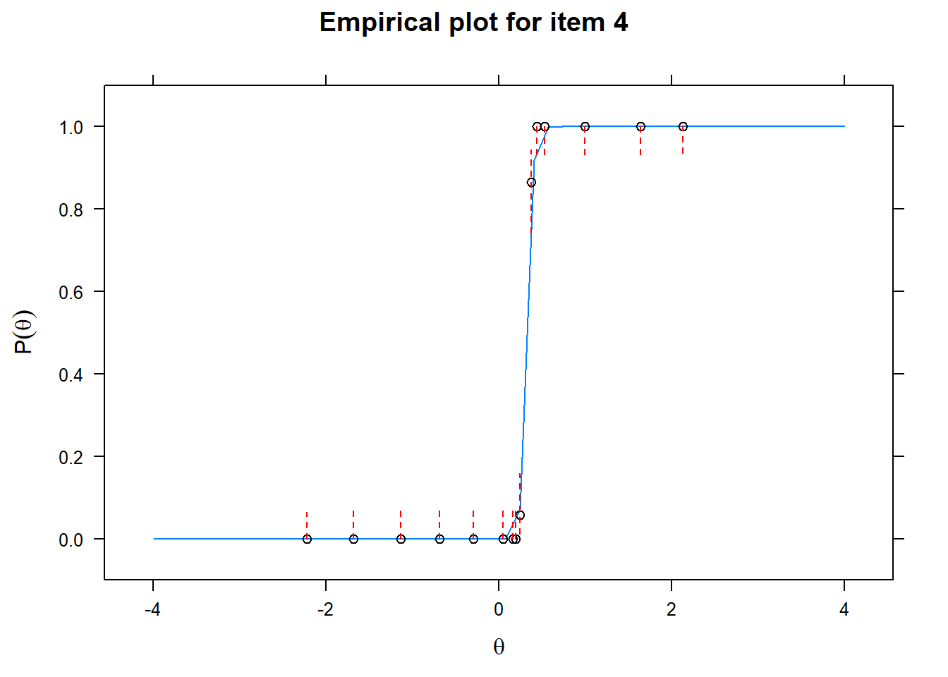
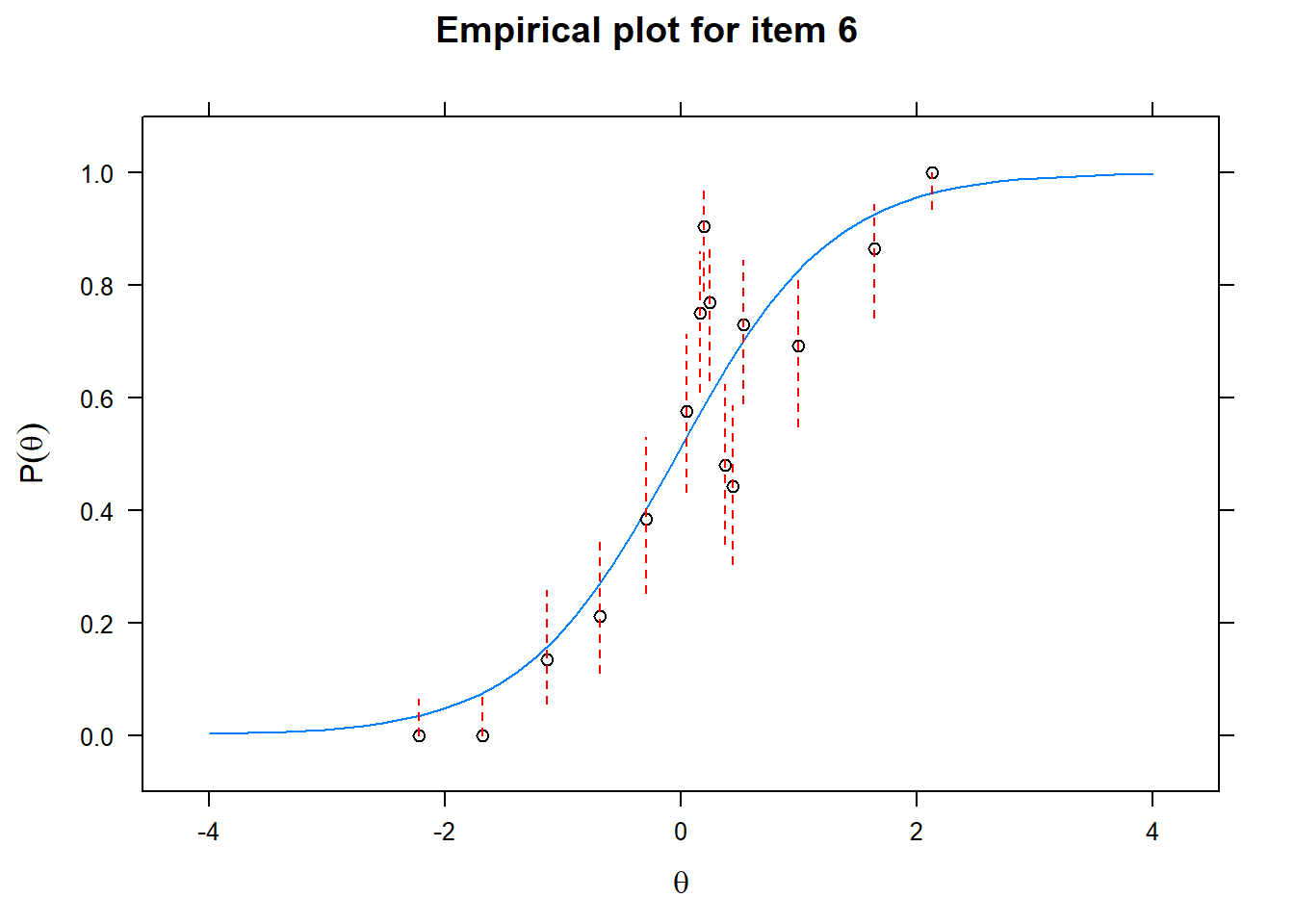
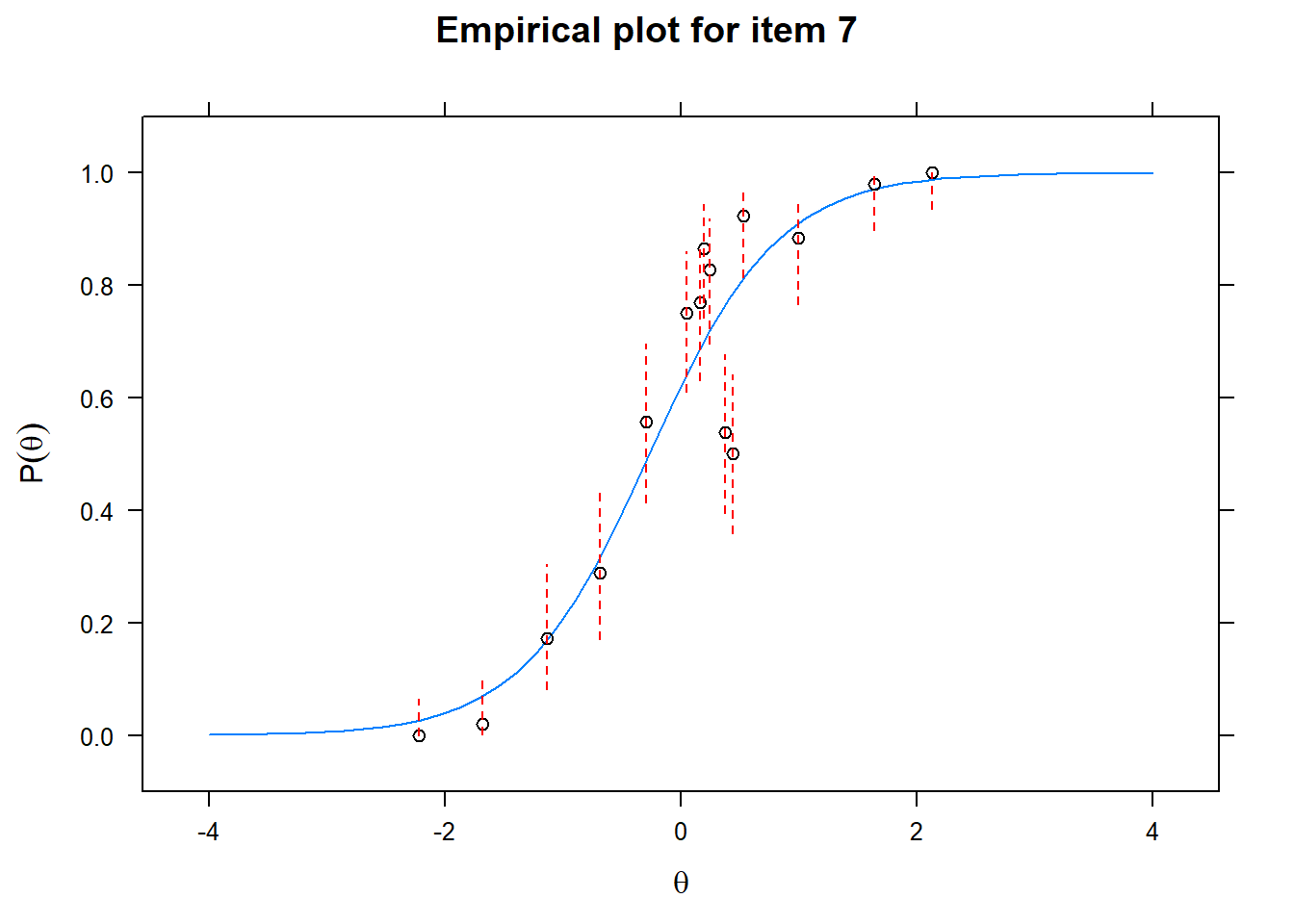
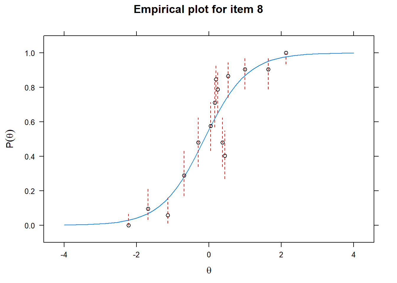
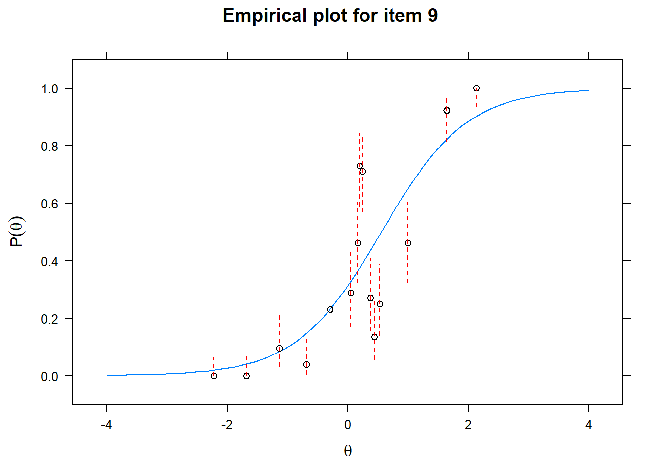
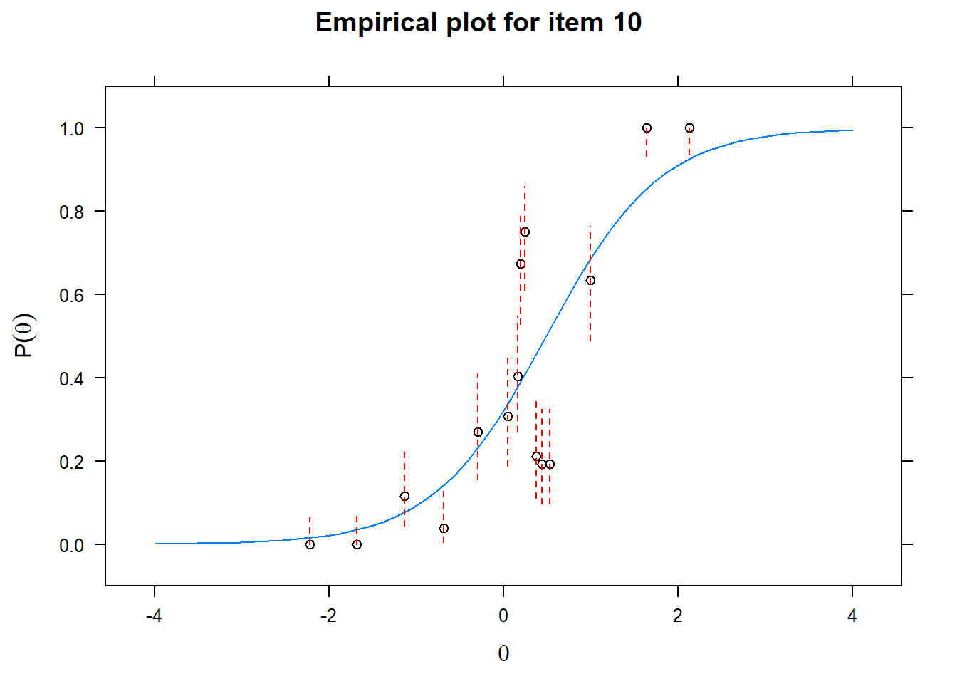
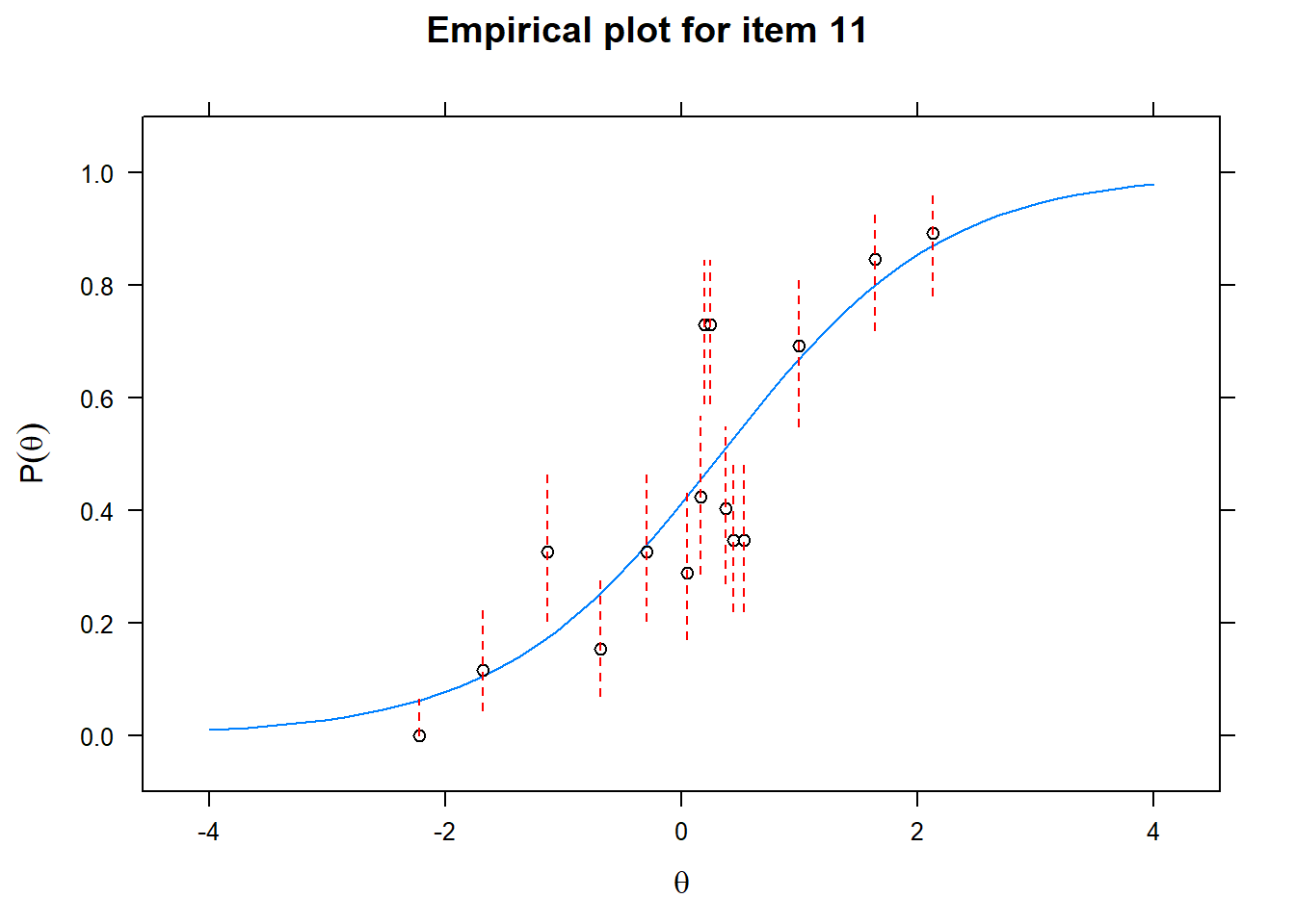
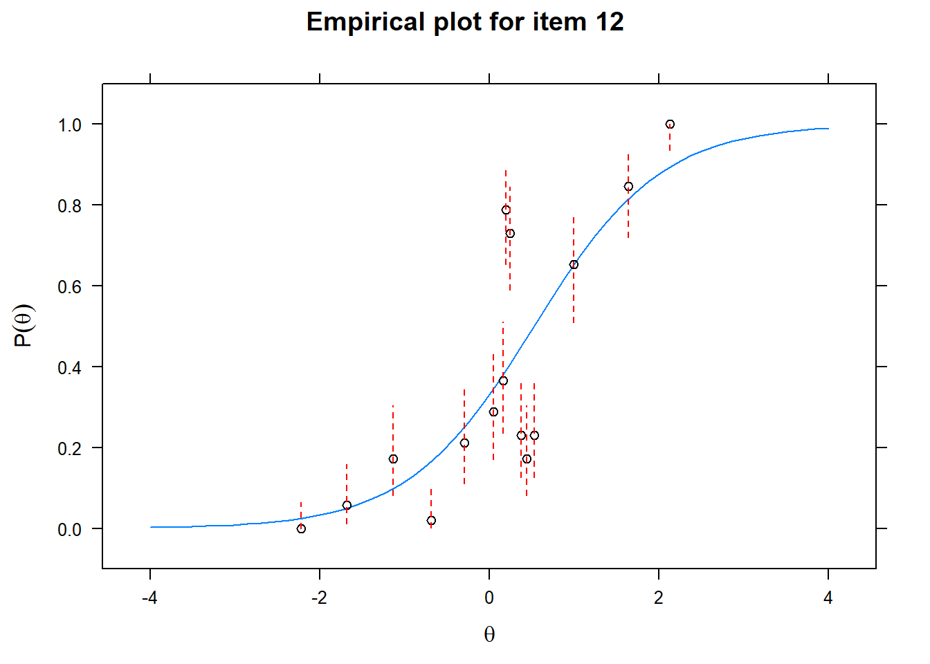
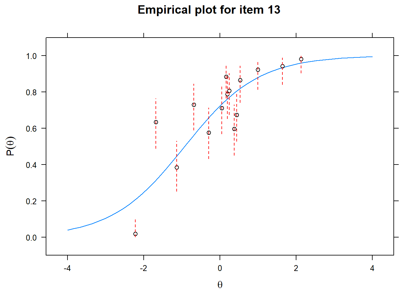
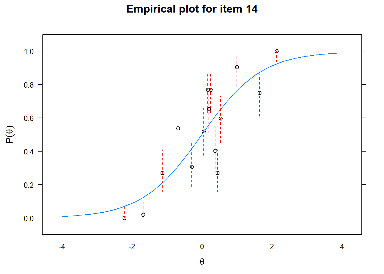
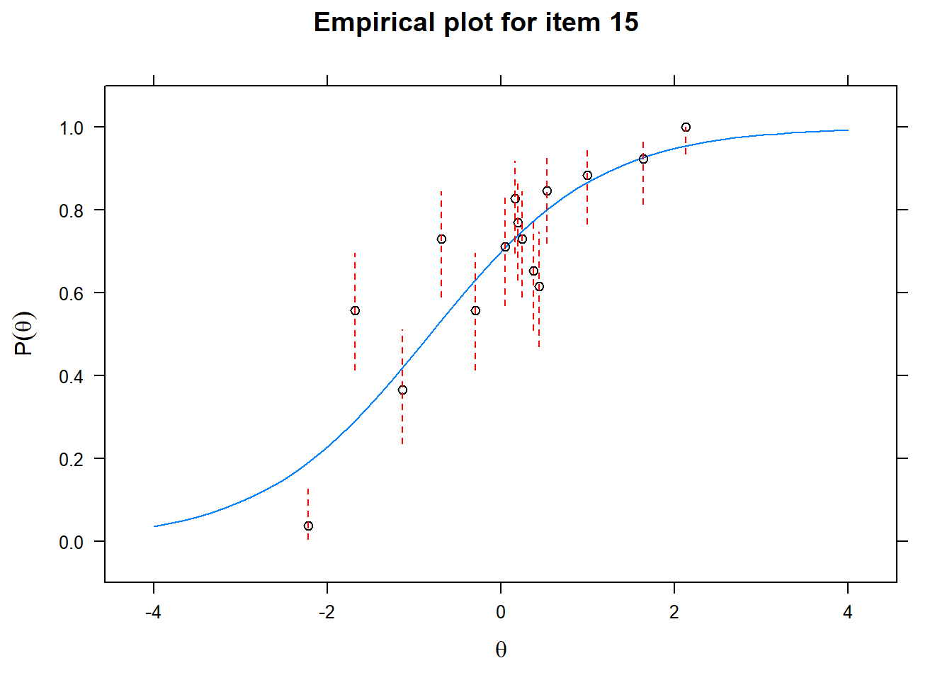
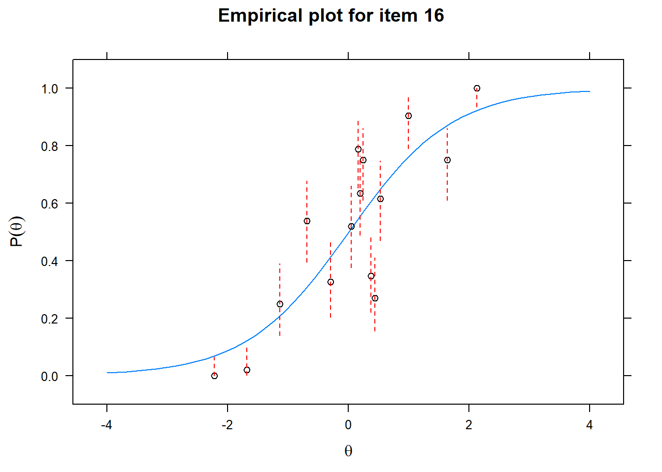First of all, the estimated models appear to fit the data reasonably well. Second, we note that questions 1-4 give an humongous amount of information for students around $θ$ = 0.2, but very little for students lower or higher in the scale. In other words, the discrimination for questions 1-4 is extreme - that is, $α$ must be very high for these questions. We pull out the $α$ parameters to confirm this observation.

fit1_coefs <- coef(fit1, 
                   simplify=T,
                   IRTpars=T)

latent_scores <- as.vector(fscores(fit1))

print(fit1_coefs$items[,1])

##        G1        G2        G3        G4        I1        I2        I3        I4 
## 19.986196 28.201574 31.570392 30.585809  1.771157  1.521330  1.837990  1.682591 
##        E1        E2        E3        E4        C1        C2        C3        C4 
##  1.416098  1.534383  1.062528  1.333830  1.036982  1.171095  1.032342  1.171904

The first four values of $α$ indeed dwarf the others.

Next, we plot a so called Wright Map, which plots the item difficulty as dots together with a histogram containing the average $θ$ scores of the students on the left. The 16 values of the dots are displayed in a table below as well.

wrightMap(latent_scores, fit1_coefs$items[,2])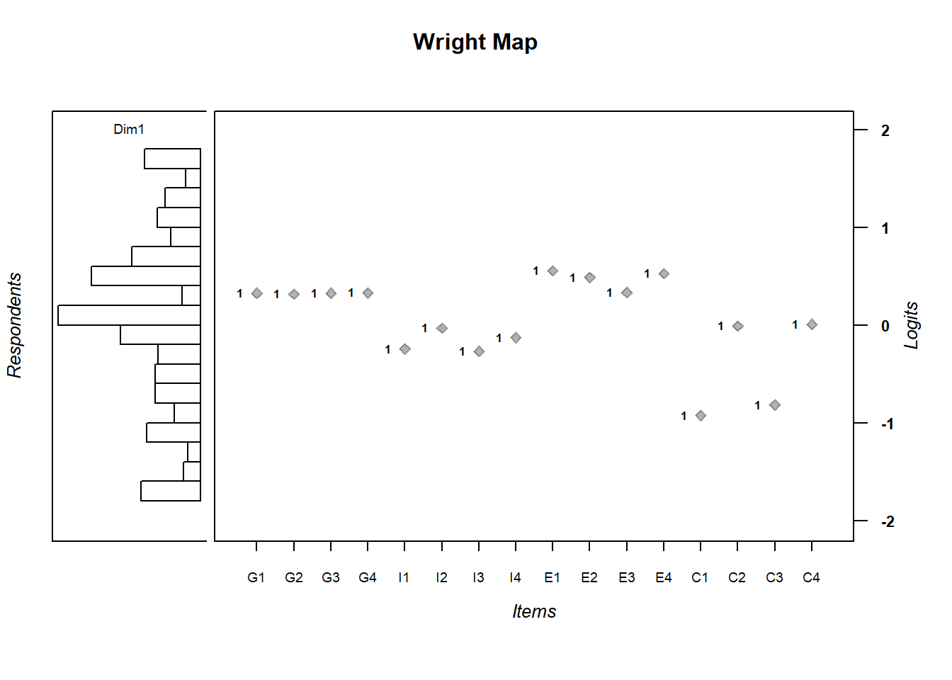

##            [,1]
## G1  0.326588911
## G2  0.314661307
## G3  0.326976070
## G4  0.328789665
## I1 -0.244611823
## I2 -0.031869313
## I3 -0.267937550
## I4 -0.128697944
## E1  0.555965627
## E2  0.487270267
## E3  0.333455121
## E4  0.526004490
## C1 -0.925990531
## C2 -0.009478124
## C3 -0.817776980
## C4  0.006975076

We see that the average $θ$ scores of students are pretty uniformly distributed. The item difficulty is clumped in the center though. This is probably what Rohrer and his team intended. The questions are unambiguous and all test a basic level of understanding. As a first field test of interleaving in math, it makes sense to start with basic questions to reduce noise. Whether interleaving benefits higher level problem solving, where several pieces of information must be integrated, can be investigated later. This observation has consequences for the interpretation of the study results though.

Next, we want to get a feel for the information that each of the items contributes. We therefore plot the item information function.

plot(fit1, type='infotrace')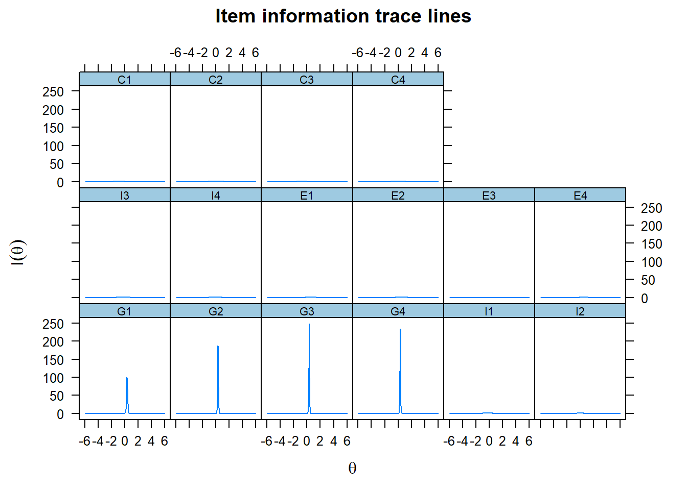

We only see the information curve for the first four items G1-G4, because their curves are so extremely steep. We therefore adjust the scale on the y-axis to get a better picture of the contribution of the other items.

plot(fit1, type='infotrace',ylim=c(0,1))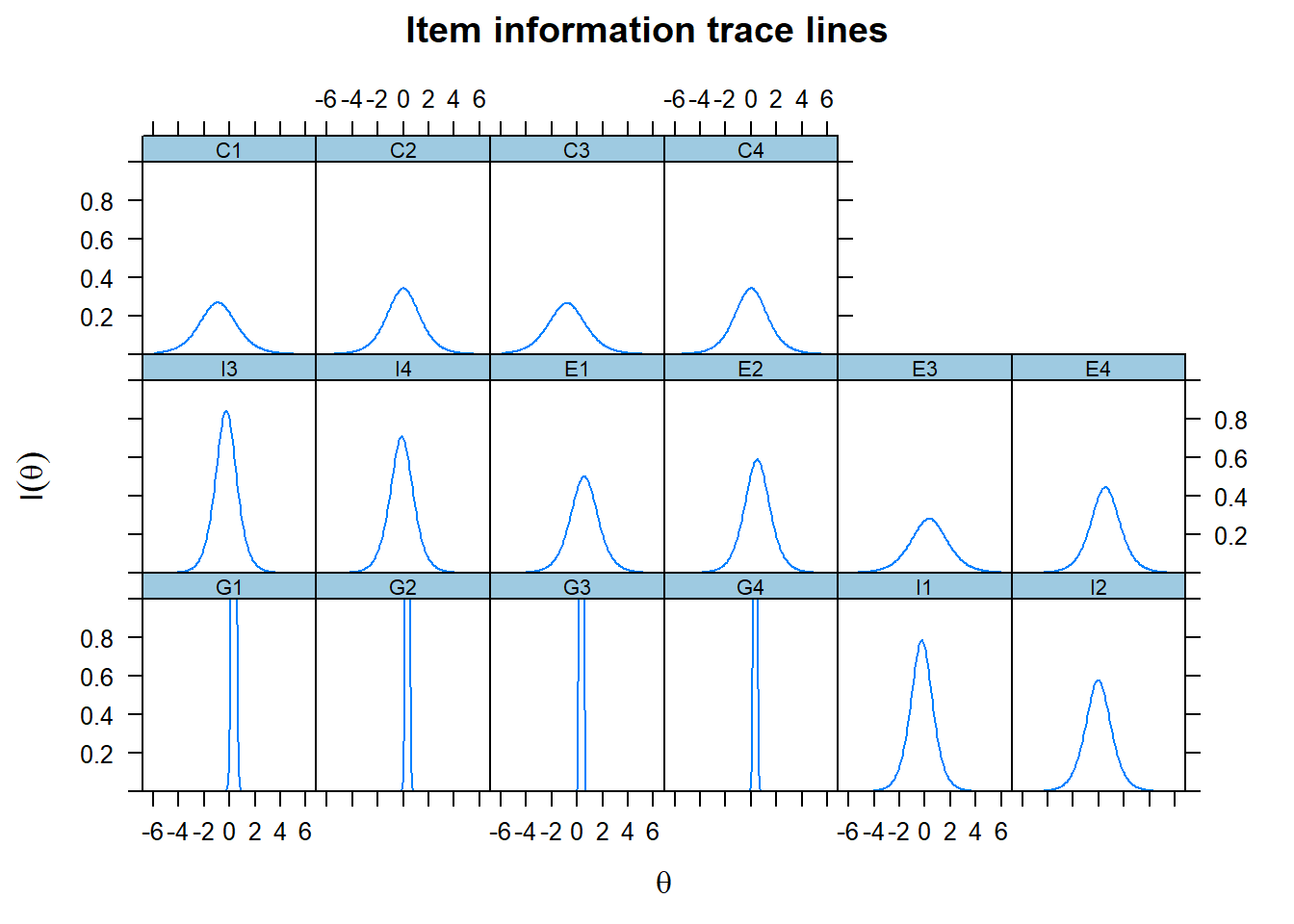

As the test information function simply sums the item information functions, it makes sense to plot the latter in one graph. We see the contribution of each item, given the level of $θ$ , where we of course note that the extreme contribution of the first four items for central values of $θ$ are cut off again.

plot(fit1, type='infotrace', facet_items=F,ylim=c(0,1))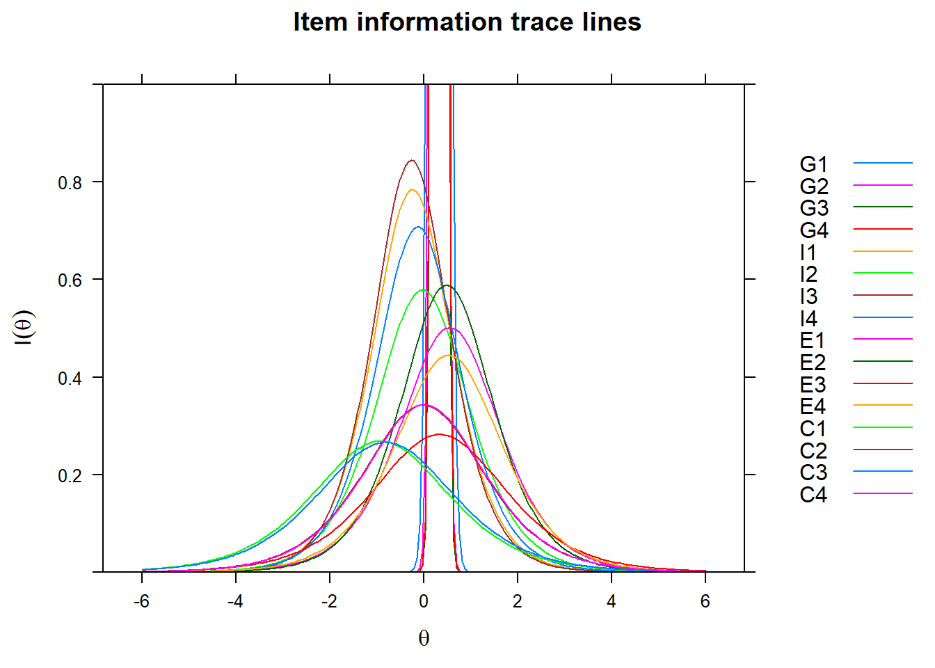

We are now ready to plot the standard error, given a level of $θ$ . The blue graph displays the information but only shows the contribution of the first four items because the scale is so large.

plot(fit1, type='infoSE')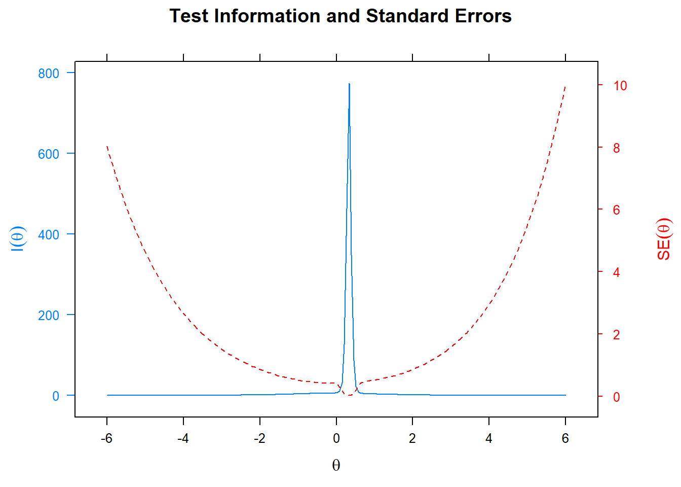

This is a plot that comes with the mirt package, like all of the others. I am not sure whether double y-axis are ever a good idea, but here it is instructive at least to see the relation between the information and the standard error. We note that standard errors are extremely small for students with average $θ$ latent ability levels, but rather quickly go up as we move up or down the ability scale.

So what have we gained by using IRT? To begin to answer this question, we plot the latent ability scores against the standardized sum of points scored on the test.

rohrer_irt <- rohrer %>% mutate(irt =latent_scores,
                                total = rowSums(.[grep("[A-Z]+[1-4]", names(.))]),
                                stand_total = (total - mean(total))/sd(total[Group == "block"]))

rohrer_irt %>% ggplot(aes(x=stand_total, y=irt)) + 
  geom_point() +
  labs(x = "raw point score",
    y = quote(theta))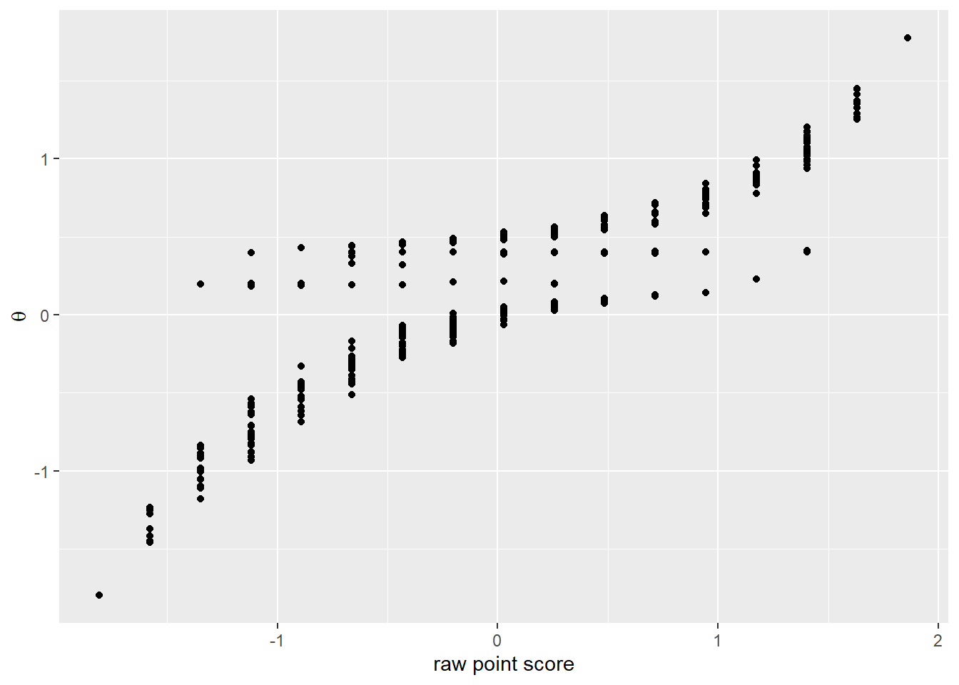

We notice a correlation, but also observe that the IRT model pulls $θ$ scores to the center. Why does it do so? The reason is that the extreme $α$ values of the first four items punish deviations from the mean difficulty of $θ$ for these items very harshly. And the mean $θ$ for these items is close to the average difficulty. If we leave out the first four items, the score align nicely again.

quest2 <- rohrer %>% select(I1:C4) %>% 
  as.data.frame()

fit2 <- mirt(quest2,
             1,                  
             itemtype = '2PL')

latent_scores2 <- as.vector(fscores(fit2))

quest2 %>% 
  mutate(irt =latent_scores2,
                                total = rowSums(.[grep("[A-Z]+[1-4]", names(.))]),
                                stand_total = (total - mean(total))/sd(total)) %>% 
  ggplot(aes(x=stand_total, y=irt)) + 
  geom_point() + 
  labs(x = "raw point score",
    y = quote(theta))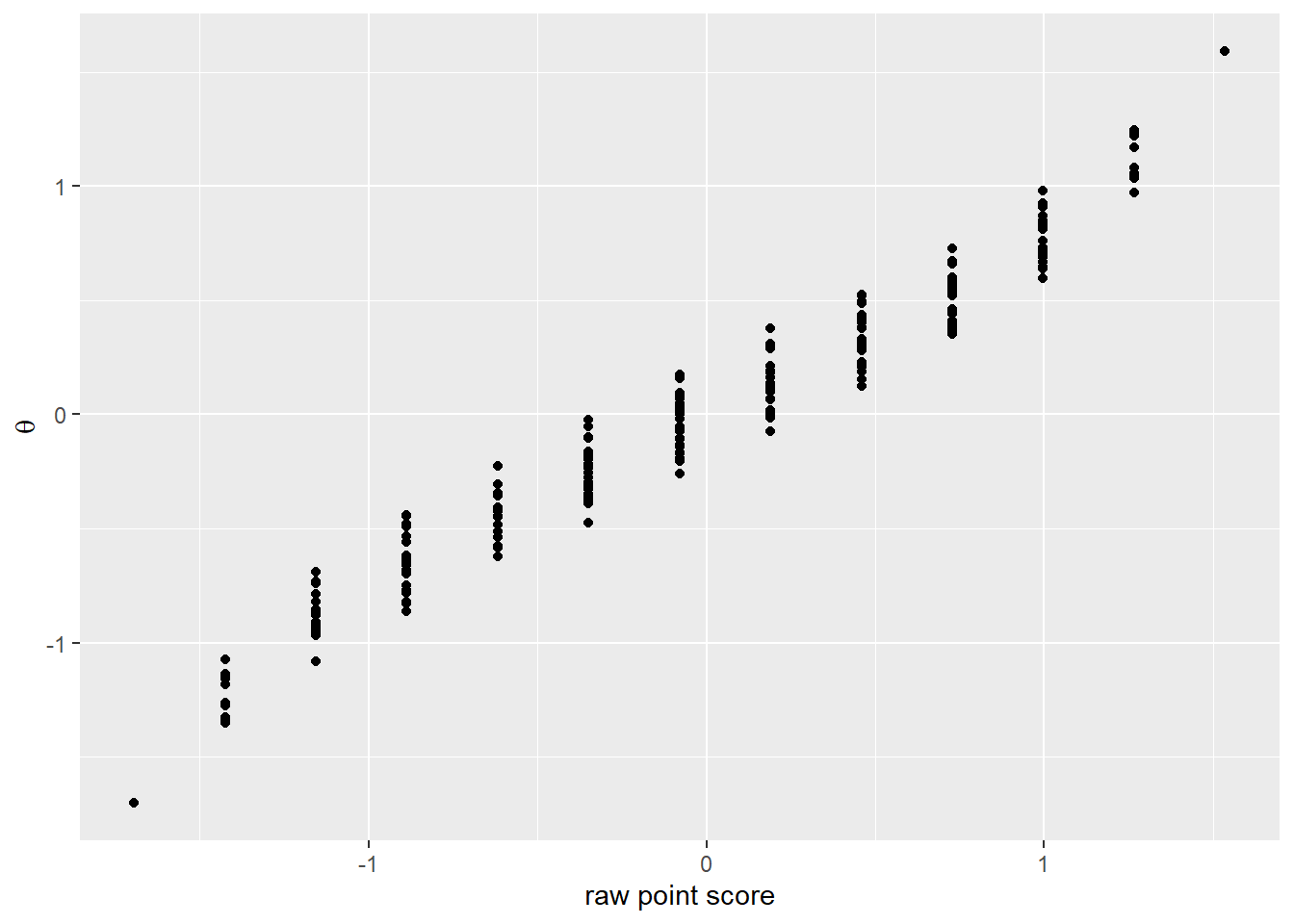

So the IRT model can’t handle the first four question on the test. Visually we noted in the first post that the responses were binary - all wrong or all right. So it’s not that surprising that the IRT model has difficulty mapping them on a continuous scale. They shouldn’t be.

Leaving out the first four items does mean we loose information though, as can be seen when we compare the plot of the standard errors with the plot of the standard error for the full model with all the items.

plot(fit2, type='infoSE')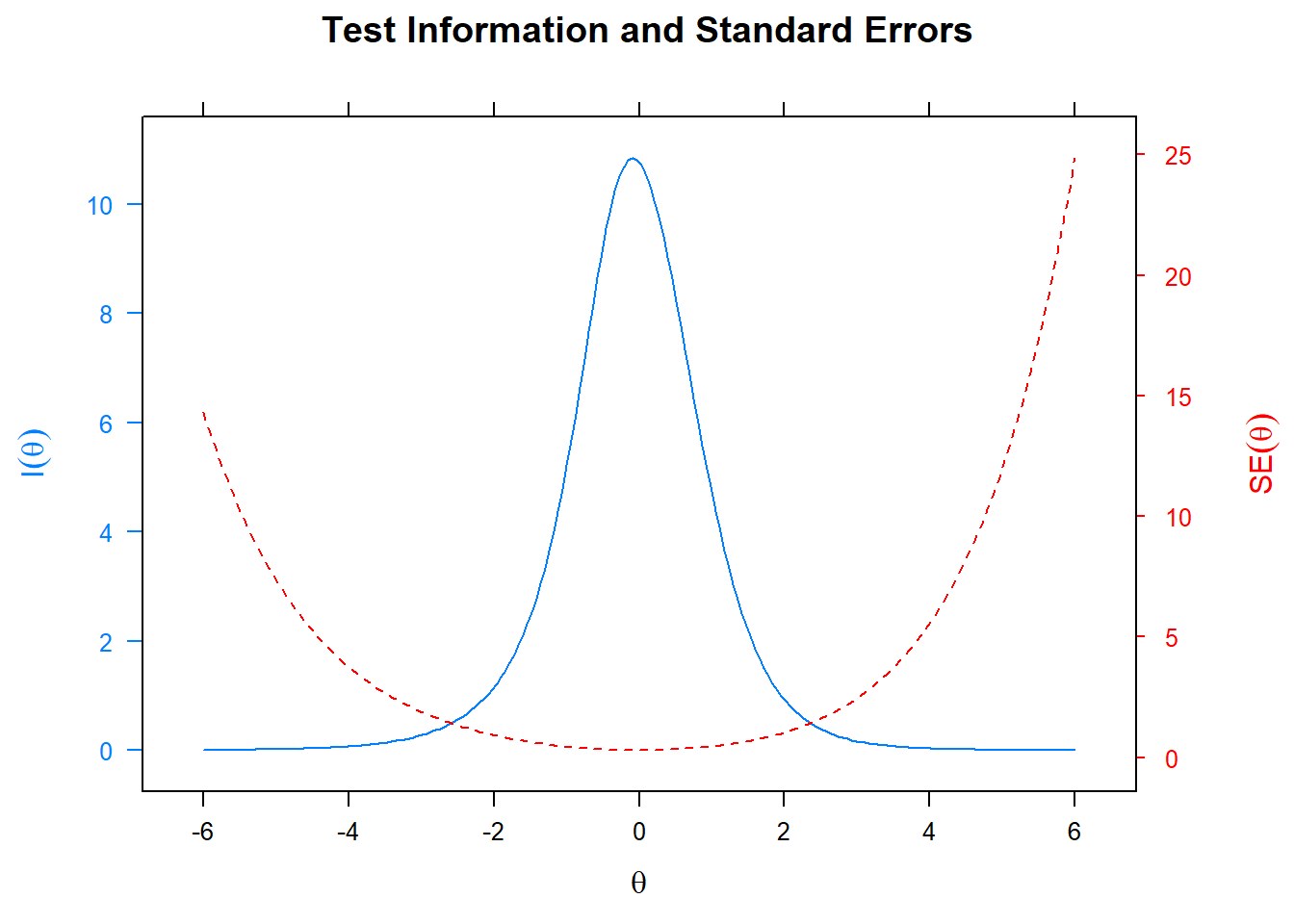

A separate issue is whether we are justified in treating the $θ$ scores as unidimensional. We knew this assumption was false, as four different domains were tested. This could all be explored with factor analysis, which we may do in a later post, which could result in the conclusion that there are really multiple abilities that are tested. But do we want to decouple solving equations from building a linear equation? We test math comprehensively and care about an integrated set of math abilities. Presumably, that is why we give a single final test and one mark. There is something to be said for both points of view, so it makes sense to pursue both lines of reasoning - one dimensional and multi dimensional analysis - in a subsequent post.

Another question is how we can use IRT to estimate the difference between the two groups in the Rohrer study, which is what we are ultimately concerned with. This question will also be taken up in a future post.

Mixing up Math: Item Response Theory (part 3)

Item Response Theory

Analysis of the Test

Edi Terlaak